Welcome! In this demo, we will explore GitHub, reproducible workflows, and data visualisation using a small dataset of birds.
Introduction
GitHub & GitLab are platforms for version control and collaboration using Git. They allow you to track changes, work with collaborators, and host your projects online.
We use a simple dataset (birds_map.csv) as an example. Yours will be much more Awesome!
Code
birds_map <-read.csv("../data/birds_map.csv",header=T,sep=",")# Display the first few rows nicely in HTMLknitr::kable(head(birds_map), format ="html")
StudyID
Species
Developmental_mode
Study_area
Lat_study_area
Long_study_area
rayyan-123815011
Ficedula albicollis
altricial
Gotland; Sweden
57.17
18.33
rayyan-123815011
Ficedula albicollis
altricial
Gotland; Sweden
57.17
18.33
rayyan-123815011
Ficedula albicollis
altricial
Gotland; Sweden
57.17
18.33
rayyan-123815011
Ficedula albicollis
altricial
Gotland; Sweden
57.17
18.33
rayyan-123815144
Tachycineta bicolor
altricial
Watauga County; USA
36.20
-81.67
rayyan-123815659
Hirundo rustica
altricial
Badajoz; Spain
NA
NA
Data Preparation
We extract Location and Country from the Study_area column and create a summary dataset.
Code
# Split Study_area into Location and Countrybirds_map[c("Location", "Country")] <-str_split_fixed(birds_map$Study_area, ";", 2)# Keep one row per unique locationbirds_map_unique <- birds_map[!duplicated(birds_map$Location), ]# Add a size variable for plottingbirds_map_unique <-ddply(birds_map_unique, "Location", transform, size =count(Location))birds_map_unique$size1 <- birds_map_unique$size.freq +1
Map Visualization
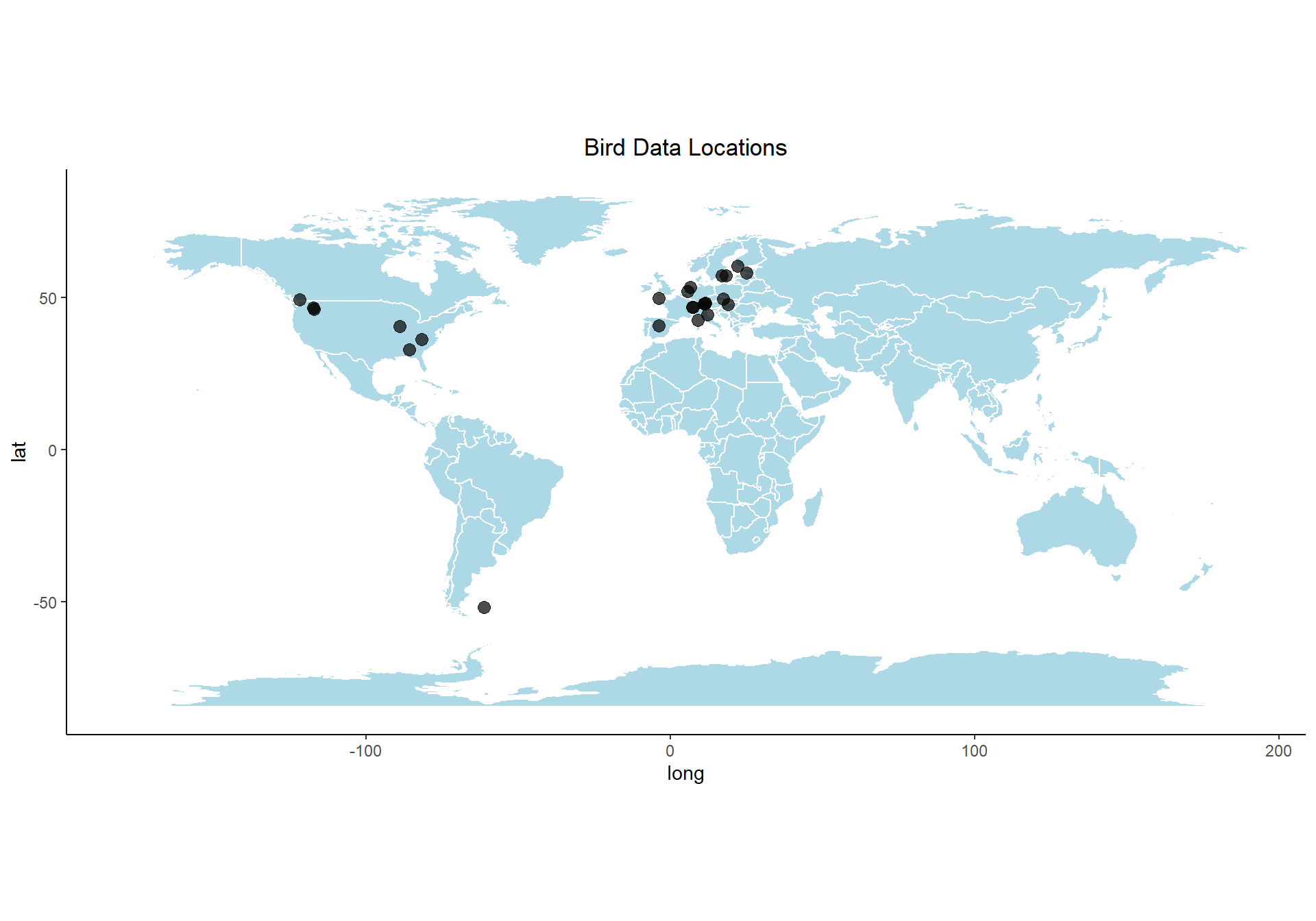
Let’s plot something, because we love plots. We create a world map with points showing data locations.
Code
# World map coordinatesworld_coordinates <-map_data("world")# Remove rows with missing coordinatesbirds_map_unique <-subset(birds_map_unique,!is.na(Long_study_area) &!is.na(Lat_study_area))# Create world map using geom_polygonfig_map <-ggplot() +geom_polygon(data = world_coordinates,aes(x = long, y = lat, group = group),color ="white", fill ="lightblue" ) +geom_point(data = birds_map_unique,aes(x = Long_study_area, y = Lat_study_area),color ="black", alpha =0.7,size =3 ) +coord_quickmap() +# correct aspect ratiotheme_classic() +labs(title ="Bird Data Locations") +theme(legend.position ="none",plot.title =element_text(hjust =0.5) )fig_map
The map shows the geographic locations of the bird data analyzed in Do Egg Hormones Have Fitness Consequences in Wild Birds? A Systematic Review and Meta-Analysis by L. Mentesana, M. Hau, P. B. D’Amelio, N. M. Adreani, A. Sánchez-Tójar (2025).
The original dataset can be found in the Zenodo repository associated with the publication:
---title: "The Best Ever Paper Written"authors: "You and Your Awesome Collaborators"project: type: website output-dir: docs # this is relative to project root, not the .qmd fileformat: html: toc: true toc-location: left code-fold: true code-tools: true code-block-bg: true code-block-border-left: "#31BAE9" code-copy: hover code-overflow: wrap---# Importing the most amazing datasetWelcome! In this demo, we will explore **GitHub, reproducible workflows, and data visualisation** using a small dataset of birds.# Introduction**GitHub & GitLab** are platforms for version control and collaboration using Git. They allow you to track changes, work with collaborators, and host your projects online.**FAIR principles** ([Wilkinson et al. 2016](https://doi.org/10.1038/sdata.2016.18)):- **F**indable: easy to locate your data/code - **A**ccessible: public and retrievable (you need a DOI!)- **I**nteroperable: standard formats and conventions - **R**eusable: documented, licensed, ready for reuseThis repository illustrates both:- A clear project structure (`data/`, `code/`, `figures/`, `docs/`) - Reproducible analysis using Quarto - FAIR metadata in the READMEFor similar guidelines for code, see [Ivimey-Cook et al. 2026](https://doi.org/10.32942/X2D93K) and for additional information on reproducible repositories, see [Pick et al. 2025](https://doi.org/10.32942/X24P8S)```{r Setup, include=FALSE}# Clear memoryrm(list =ls()) # Load required packages (installs pacman if needed)if (!require("pacman")) install.packages("pacman")pacman::p_load(ggplot2, plyr, stringr, knitr, maps)```# Importing the most amazing datasetWe use a simple dataset (`birds_map.csv`) as an example. Yours will be much more Awesome!```{r}birds_map <-read.csv("../data/birds_map.csv",header=T,sep=",")# Display the first few rows nicely in HTMLknitr::kable(head(birds_map), format ="html")```# Data PreparationWe extract **Location** and **Country** from the `Study_area` column and create a summary dataset.```{r}# Split Study_area into Location and Countrybirds_map[c("Location", "Country")] <-str_split_fixed(birds_map$Study_area, ";", 2)# Keep one row per unique locationbirds_map_unique <- birds_map[!duplicated(birds_map$Location), ]# Add a size variable for plottingbirds_map_unique <-ddply(birds_map_unique, "Location", transform, size =count(Location))birds_map_unique$size1 <- birds_map_unique$size.freq +1```# Map VisualizationLet's plot something, because we love plots. We create a world map with points showing data locations.```{r, warning=FALSE, fig.width=10, fig.height=7}# World map coordinatesworld_coordinates <-map_data("world")# Remove rows with missing coordinatesbirds_map_unique <-subset(birds_map_unique,!is.na(Long_study_area) &!is.na(Lat_study_area))# Create world map using geom_polygonfig_map <-ggplot() +geom_polygon(data = world_coordinates,aes(x = long, y = lat, group = group),color ="white", fill ="lightblue" ) +geom_point(data = birds_map_unique,aes(x = Long_study_area, y = Lat_study_area),color ="black", alpha =0.7,size =3 ) +coord_quickmap() +# correct aspect ratiotheme_classic() +labs(title ="Bird Data Locations") +theme(legend.position ="none",plot.title =element_text(hjust =0.5) )fig_map```The map shows the geographic locations of the bird data analyzed in **Do Egg Hormones Have Fitness Consequences in Wild Birds? A Systematic Review and Meta-Analysis** by *L. Mentesana, M. Hau, P. B. D'Amelio, N. M. Adreani, A. Sánchez-Tójar (2025)*. The original dataset can be found in the Zenodo repository associated with the publication: Publication: [Mentesana et al. 2025, Ecology Letters 28: e70100](https://doi.org/10.1111/ele.70100)Zenodo repository: [DOI: 10.5281/zenodo.14930059](https://doi.org/10.5281/zenodo.14930059)# ReproducibilityAlways include **R session info** for reproducibility.```{r}sessionInfo()```